Cell references often confuse Excel users no matter how simple they may sound.
Be it Cell A1 or Cell XFD1048576. How are these cell references made?🤔
The guide below will teach you this and much more. So jump right in.
And as you go, download our free sample workbook here to practice along the guide.
Table of Contents
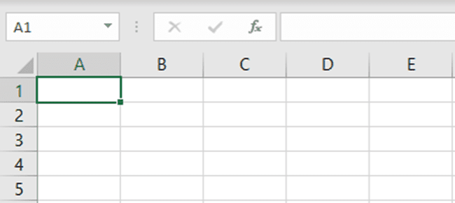
Cell references are like the name of cells. A cell reference is alphanumeric; it consists of an alphabet and a number. 🔠
Where do this alphabet and number come from? Here is what a worksheet in Excel looks like (A two-dimensional window with rows and columns).
Columns in Excel are denoted by alphabet. Whereas rows in Excel are denoted by numbers.
A cell is formed at the intersection of a row and a column. It is then named as a combination of that row and column.
For example, in the image below the highlighted cell forms at the intersection of Column B and Row 2.
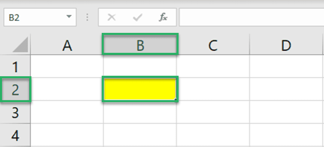
The highlighted cell is referred to as Cell B2 (Column B and row 2).
Similarly, drag your worksheet to the end to see if even the last cell (Cell XFD1048576) is referred to the same way.
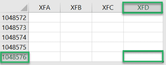
It is formed at the intersection of Column XFD and Row 1048576.
Pro Tip!
Did you know? There are a total of 16,384 columns in Excel. And the total number of rows in Excel is 1,048,576. 💯
Cell references make your Excel jobs unbelievably easy. You can use them everywhere and the best thing – as you move the formulas, the cell reference automatically adjusts.
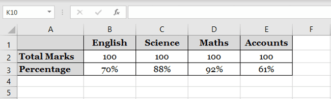
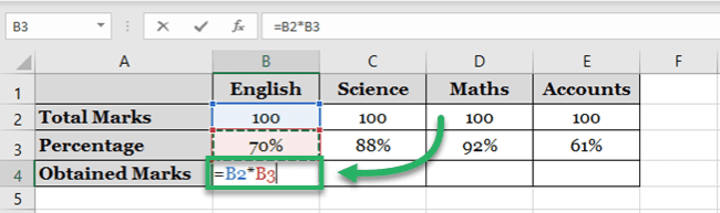
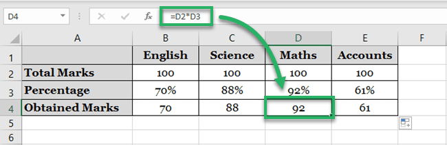
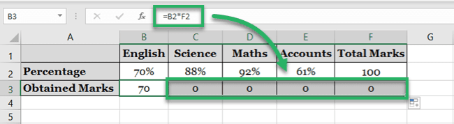
The image shows the total marks for each subject in Row 2. The percentage marks acquired by a student in each of these subjects is in Row 3.
Let’s quickly find the marks scored in each subject.
Write the formula in Cell B4 as follows:
= B2 * B3
 Formula with relative cell reference" width="650" height="193" />
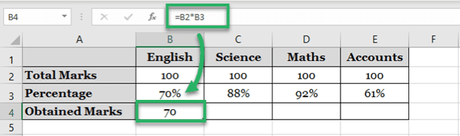
We are multiplying Cell B2 (Total marks) by Cell B3 (Percentage). Excel calculates the obtained marks in English.
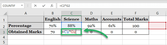
Let’s calculate the same for the remaining subjects. But don’t waste time writing the respective formula for each subject.
Drag and drop the formula in Cell B4 to the remaining cells.
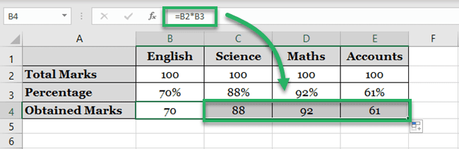
Excel calculates the obtained marks for all the remaining subjects.
But what has Excel done?
When formulas are moved across cells, Excel changes the relative cell references based on the relative rows/columns.
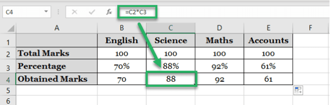
For example, the above formula when copied from Column B to C becomes:
= C2 * C3
Move it from Column C to Column D to see it changes as follows.
= D2 * D3
That way, you do not have to write formulas unique to each cell.
You can put together a single formula for one cell and copy/paste it to the others. Excel will automatically update the relative cell references. 💪
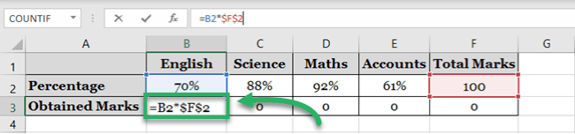
What if the above data changes as shown below?
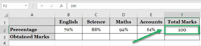
The data remains the same. However, marks for each of the subjects are not mentioned now. Instead, we have the total marks in Cell F2 only.
To calculate the marks obtained in English, write the formula below.
= B2 * F2
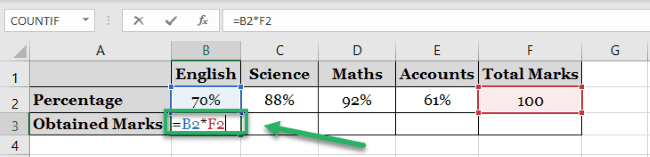
B2 consists of the percentage marks obtained in English. At the same time, Cell F2 consists of the total marks for all the subjects.
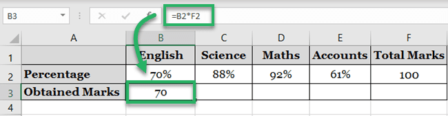
Excel calculates the marks obtained in English as below.
Can we move the same formula (drag and drop it) for the remaining subjects?
The results are bizarre. What has Excel done?
The cell references were relative. As we moved it from one column to another, Excel changed the column reference from F2 to G2. G2 is an empty cell, so, Excel returns zero.
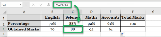
In such a case, we don’t want Excel to change the cell reference (F2) every time the formula is moved. We want to keep it constant.
However, we want the cell reference for percentages to change every time the formula is moved.
Write the formula as follows.
= B2 * $F$2
We have changed the relative reference of Cell F2 into an absolute reference of $F$2.
Unlike relative cell references, an absolute cell reference has a dollar symbol before the column and the row reference. Like $A$1.
However, the cell reference B2 is still the same. This is because we only want to fix the cell reference $F$2 but not B2.

Kasper Langmann , Microsoft Office Specialist
Drag and move it across all the columns
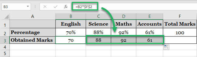
Excel calculates the obtained marks for all the subjects.
This time Excel updated the formula for each next column by changing the cell reference of B2 but not F2.
For example, when moved to Column C, Excel changes the formula as below.
So, the formula changes from:
=INDEX(D:D,MATCH(G2,A:A,0))
=INDEX(D:D,MATCH(1,A:A,0))
The “theory” behind this is not as simple as changing the lookup value.
Since you’re changing the formula from a normal one to an array formula, the structure of the formula changes a bit as well. By changing the lookup value to 1, you’re not actually telling the MATCH function to search for the number 1 in the lookup array (last name column).
Pro Tip!
To change any reference into an absolute cell reference, click on that cell reference in the formula bar and press the F4 key.